Thermal Systems [Part 2]

MATLAB Simulation of the Heating

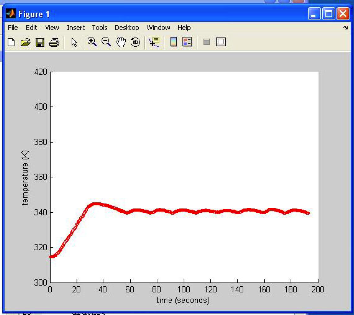
For the thermal challenges, we first had to calculate the physical constants of the heating system. In order to do so, we had to get a graph (temperature vs. time) of our thermometer in the process of heating up. Here is the graph that we used to calculate the constant.



To calculate C, we used the interval between time=20 and time=40 because there weren't much fluctuation and, therefore, was more reliable than the other. Also, because we were told to do so. Here is the equation we used to calculate C:

Change in temperature = 20 degrees
C = heat capacity = dE/dT
dE = P * dt = 6.48 * 20 = 129.6
C = 129.6 / 20
C = 6.48

To calculate Rth, we used the whole interval for change in temperature and applied the values to the equation below:

dT = 80 degrees
Rth = dT / dE
dE = P = 6.48
Rth = dT/dE = 80/6.48
Rth = 12.34

Below is our graph of simulation heatsim.m.

We believe that the simulation agrees almost with our experimental results in that it starts and end in similar places and that it has the similar curve to it. However, we found that when we saw some delay in the beginning of our heating system in experiment, the simulation did not. Right off from the beginning (intervals from time=0 to time=20), the temperature continued to rise without any delay.

Bang-Bang Control

The image below shows our graph to simulation for Bang-Bang Control:



The image below shows our graph to experimental results to Bang-Bang Control.



Our implementation was different from the simulation in that it had gentler oscillations and gradual changes in slope each time.